Week 2: Visualizing Hydrogen Atomic Orbitals
Overview and Objectives
The world of scientific programming with Python begins with the SciPy ecosystem of libraries, which provide a wide variety of data structures, algorithms, and visualization tools that allow a user to get results quickly. The ecosystem consists of 6 main parts, and we will touch on most of them in this course:
- NumPy: Efficient implementations of N-dimensional arrays
- SciPy: Common scientific quantities, functions, and algorithms
- matplotlib: Plotting library for 1D, 2D, and 3D data
- iPython: An interactive python console with extra features
- SymPy: Library for symbolic mathematics
- pandas: Library with extra data structures and analysis tools
This week we will be making a variety of plots involving the atomic orbitals of the hydrogen atom. Often, the ability to visualize functions or data is the first step toward interpreting and understanding it, and it is especially important for communicating it to others. Our goal for this week is to learn the basics of data visualization with matplotlib. We will be using matplotlib extensively throughout the quarter, and it is likely something you will come back to often even after this class. Along the way, we will start to learn about using NumPy arrays and parts of the SciPy library.
Background
In General Chemistry, you learned about the \(s\), \(p\), \(d\), \(\ldots\) orbitals of the hydrogen atom, and their associated quantum numbers:
- \(n\): The “principal” quantum number that determines the electron’s “shell” and its energy. Allowed values are positive nonzero integers: \(1, 2, 3, \ldots.\)
- \(\ell\): The orbital angular momentum quantum number, which determines the orbital’s shape \(s, p, d, \ldots.\) Allowed values are \(0, 1, \ldots, n-1.\)
- \(m\): The orbital angular momentum projection quantum number, which determines the orbital’s orientation. Allowed values go from \(+\ell\) to \(-\ell\) in steps of 1.
These numbers come from a quantum mechanical treatment of the hydrogen atom: they are the solutions to the Schrödinger equation
\[ \hat{\mathbf H}\psi = E\psi \]
In this equation, \(\hat{\mathbf H}\) is the Hamiltonian operator, which is the quantum mechanical representation of the energy of the system, \(\psi\) is the wavefunction, the physical state of the system, and \(E\) is the energy of the system. A hydrogen atom consists of a proton whose mass is \(m_p\) and charge \(+e\) that is being orbited by an electron of mass \(m_e\) and charge \(-e\). If the proton is placed at the origin of the coordinate system, to a very good approximation the energy of the system is just given by the kinetic energy of the electron orbiting the stationary proton and the potential energy due to the electrostatic interaction between the negative and positive charges. Using the quantum mechanical operators for position and momentum (beyond the scope of this course!), the Hamiltonian for the hydrogen atom in SI units is
\[ \hat{\mathbf H} = -\frac{\hbar^2}{2m_e}\nabla^2 - \frac{e^2}{4\pi\epsilon_0 d}.\]
- \(\hbar \equiv h/2\pi\) is Planck’s constant divided by \(2\pi\).
- \(m_e\) is the mass of the electron.
- \(\nabla^2 \equiv \frac{\partial^2}{\partial x^2} + \frac{\partial^2}{\partial y^2} + \frac{\partial^2}{\partial z^2} \) is proportional to the square of the quantum mechanical momentum of the electron.
- \(e\) is the fundamental unit of charge.
- \(\epsilon_0 \) is the permittivity of free space, a fundamental constant.
- \(d\) is the distance of the electron from the proton in meters. At position (x,y,z), \(d = \sqrt{x^2 + y^2 + z^2}\).
Given all the numbers above, it is much more convenient to work in atomic units (a.u.), which redefines units of length, mass, charge, and action in terms of fundamental constants.
| Dimension | Term | SI Value | SI Units | a.u. Value | a.u. Definition |
|---|---|---|---|---|---|
| action | \(\hbar\) | \(1.05457\times 10^{-34}\) | J\(\cdot\)s | 1 | \(\hbar \) |
| charge | \(e\) | \(1.602\times 10^{-19}\) | C | 1 | \(e\) |
| length | \(a_0\) | \(5.2918\times10^{-11}\) | m | 1 | \( \frac{4\pi \epsilon_0 \hbar^2}{m_e e^2} \) |
| mass | \(m_e\) | \(9.109\times 10^{-31}\) | kg | 1 | \(m_e\) |
| energy | \(E_h\) | \(4.360\times 10^{-18}\) | J | 1 | \( \frac{\hbar^2}{m_e a_0^2} \) |
The quantity \(a_0\) is called the Bohr radius, and \(E_h\) is the Hartree. In atomic units, the Hamiltonian for the hydrogen atom becomes
\[ -\frac{1}{2}\nabla^2 - \frac{1}{r} \]
where \(r\) is now the distance of the electron from the proton in units of \(a_0\). The Schrödinger equation in atomic units is
\[ -\frac{1}{2}\nabla^2\psi(x,y,z) - \frac{1}{r}\psi(x,y,z) = E\psi(x,y,z) \]
where \(x\), \(y\), and \(z\) refer to the position of the electron in units of \(a_0\), and \(E\) is the energy of the electron in Hartree. Solving this equation consists of finding combinations of energy and \(\psi\) that make the equality hold. It turns out that the easiest way to solve the equation is to convert to spherical coordinates \(r\), \(\theta\), and \(\phi\):

| Cartesian | Spherical | Domain |
|---|---|---|
| \(x = r \sin \theta \cos \phi\) | \(r = \sqrt{x^2 + y^2 + z^2} \) | \(r \in [0,\infty) \) |
| \(y = r \sin \theta \sin \phi\) | \( \theta = \arccos \frac{z}{r} = \arccos \frac{z}{\sqrt{x^2+y^2+z^2}} \) | \(\theta \in [0,\pi] \) |
| \(z = r \cos \theta \) | \( \phi = \arctan \frac{y}{x} \) | \(\phi \in [0,2\pi) \) |
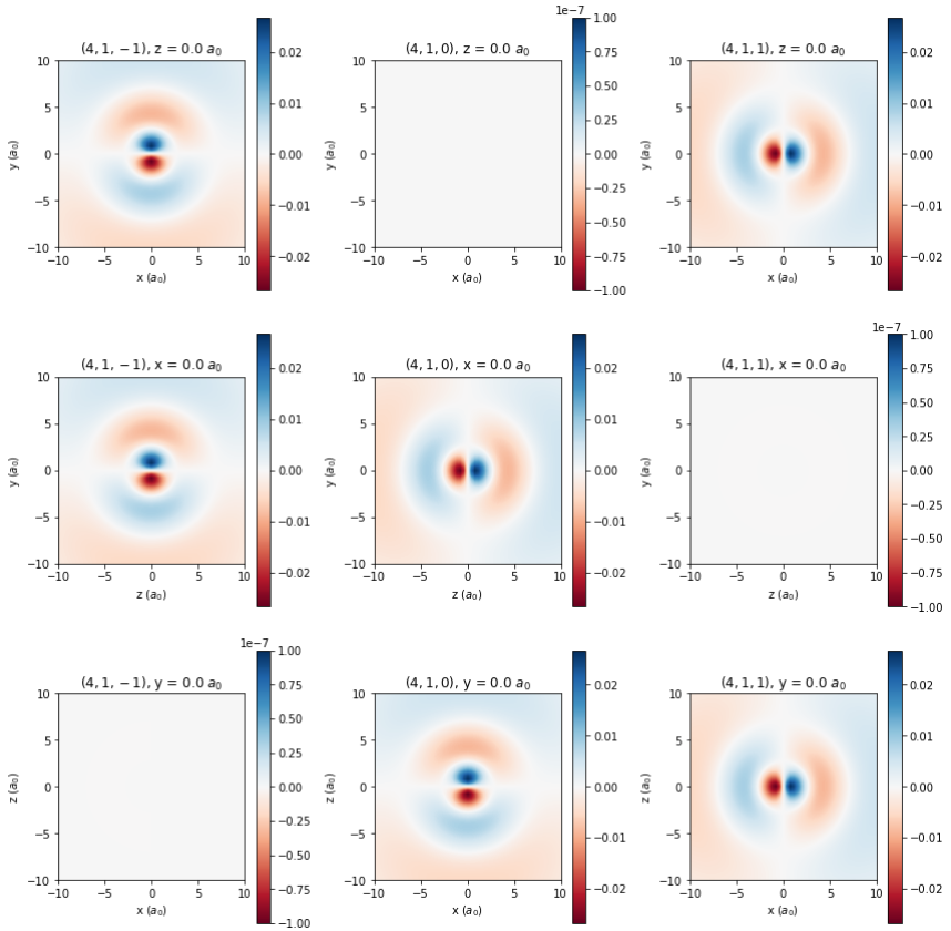
Here we are primarily concerned with the wavefunctions \(\psi\). In spherical coordinates and atomic units, the wavefunction for quantum numbers \(n\), \(\ell\), and \(m\) is:
\[\psi_{n\ell m}(r,\theta,\phi) = \sqrt{ \left( \frac{2}{n} \right)^3 \frac{ (n-\ell-1)! }{2n(n+\ell)!} } e^{-r/2} r^\ell Y_\ell^m(\theta,\phi) L^{2\ell+1}_{n-\ell-1}(r)\]
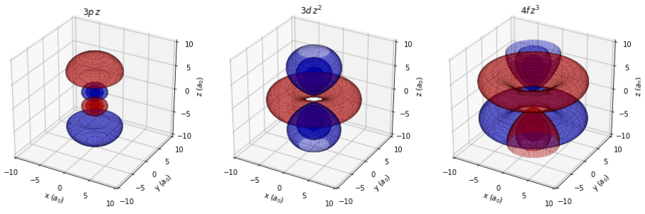
This equation introduces two new quantities, the spherical harmonics \( Y_\ell^m(\theta,\phi) \) which describe the angular dependence of the wavefunction, and the generalized Laguerre polynomials \( L_{n-\ell-1}^{2\ell+1}(r) \) which describe its radial dependence together with the \(e^{-r/2}r^\ell\) term. More details about these functions, as well as explicit forms for them, are provided at the links above. The spherical harmonics are complex-valued functions. In chemistry, it is common to convert them into real-valued functions by taking linear combinations; this will generate the normal \(p_x\), \(p_y\), and \(p_z\) orbitals that are shown in general chemistry, for instance. One easy way to do this, which we will make use of this week, is shown in the table below.
| m | Real Form |
|---|---|
| \(m < 0\) | \((-1)^m \sqrt{2}\, \text{Im}\left(Y_{\ell}^{|m|}\right) \) |
| \(m = 0\) | \(Y_\ell^0 \) |
| \(m > 0\) | \((-1)^m\sqrt{2}\, \text{Re}\left(Y_\ell^{\phantom{|}m}\right) \) |
The wavefunction for the electron in the hydrogen atom describes the probability amplitude that the electron is located at a particular point in space. In general, this can be positive, negative, real, or imaginary, and it does not have a direct classical interpretation. However, the square of the wavefunction \(|\psi^2| = \psi^*\psi \) gives the probability density that the electron is located at a point. This is a real number between 0 and 1. The probability density can be integrated over space to give the probability of finding the electron inside that volume. In Cartesian coordinates, this is:
\[ \int_{x_1}^{x_2}\int_{y_1}^{y_2}\int_{z_1}^{z_2} \psi^*(x,y,z)\psi(x,y,z)\,\text{d}x\,\text{d}y\,\text{d}z \]
and in spherical coordinates:
\[ \int_{r_1}^{r_2}\int_{\theta_1}^{\theta_2}\int_{\phi_1}^{\phi_2} \psi^*(r,\theta,\phi)\psi(r,\theta,\phi)\,r^2\sin\theta\,\text{d}r\,\text{d}\theta\,\text{d}\phi \]
Further Reading
- Using Jupyter notebooks
- Difference between python list and numpy array
- Introductory matplotlib usage
- Matplotlib gallery
- What every computer scientist should know about floating point arithmetic
- Introduction to object-oriented programming in python